Survival Analysis

Metabrick dataset is used below for demoing purposes. The dataset can be found within examples/datasets/metabrick/ folder in the LogML repo. The configuration file described below might be found in examples/configs/metabrick/survival_analysis.yaml file in the LogML repo.

Useful links:

Configuration

The following configuration file defines survival analysis for metabrick dataset:

Survival Analysis config for metabrick dataset

version:                                      0.2.6

stratification:
    - strata_id:                              cohort_1
      query:                                  'cohort == 1.0'
    - strata_id:                              cohort_2
      query:                                  'cohort == 2.0'
    - strata_id:                              cohort_3
      query:                                  'cohort == 3.0'
    - strata_id:                              cohort_4
      query:                                  'cohort == 4.0'
    - strata_id:                              cohort_5
      query:                                  'cohort == 5.0'

dataset_metadata:
    modeling_specs:
        # Overall survival setup, referenced below
        OS:
            time_column:                      overall_survival_months
            event_column:                     overall_survival
            # Interpretation of event column's values is study-specific,
            # so explicit definition of 'uncensored' is required
            event_query:                      'overall_survival == 0'

survival_analysis:
    enable:                                   True
    problems:
        # Reference to the OS modeling specification.
        OS:
            # Required transformations before proceeding to analyses.
            dataset_preprocessing:
                steps:
                    # Sample ID and stratification column are removed.
                    - transformer:            drop_columns
                      params:
                          columns_to_include:
                              - patient_id
                              - cohort

            methods:
                - method_id:                  kaplan_meier
                - method_id:                  optimal_cut_off
                - method_id:                  cox

report:
    report_structure:
        survival_analysis:
            - OS

Stratification

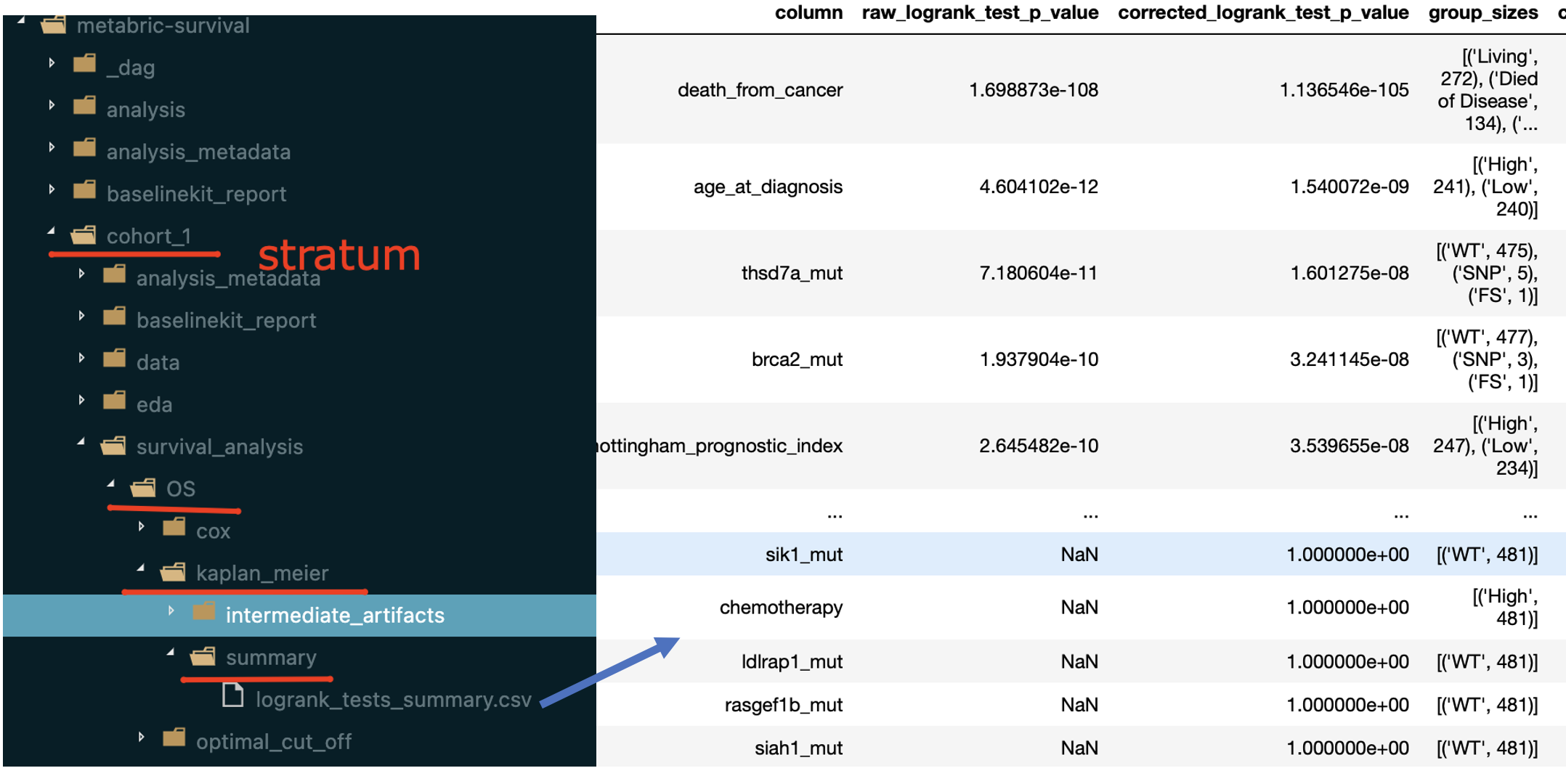
stratification section defines a set of strata for which survival analysis will be run. logml.configuration.stratification.Strata class defines each stratum.

In the example above there are 5 strata and each corresponds to some ‘cohort’ identifier.

Metadata definition

dataset_metadata/modeling_specs section defines all required survival setups (OS, PFS, etc.). For each survival setup some reasonable alias should be introduced (OS - overall survival, PFS - progression free survival) and then each alias is mapped to corresponding definition (logml.configuration.metadata.SurvivalTimeSpec).

In the example above there is the only one survival setup defined (using ‘OS’ alias) on top of the ‘overall_survival_month’ and ‘overall_survival’ columns.

Survival Analysis configuration

survival_analysis/problems section maps survival setup aliases to corresponding survival setup definitions (logml.configuration.survival_analysis.SurvivalAnalysisSetup). Each survival setup specifies how dataset should be preprocessed (dataset_preprocessing section) before applying target survival analysis methods (methods section).

report/report_structure/survival_analysis section lists all survival setup aliases for which artifacts should be included into the result report.

Univariate methods

As it was mentioned, before applying univariate methods a given dataset is preprocessed using the configured list of transformations.

Kaplan-Meier

The method consists of the following steps:

LogRank test is applied to all features (to what was left after preprocessing) - raw p-values are kept
- for numerical features median threshold is used to define ‘High’ and ‘Low’ groups
- categorical features naturally define groupings for the test
FDR correction is applied to the result raw p-values
Features are ordered according to the corrected p-values

The method can be configured using logml.survival_analysis.extractors.kaplan_meier.KaplanMeierSAParams class using params section.

The result report contains the following artifacts:

table with features ranked by FDR-corrected p-values from LogRank tests

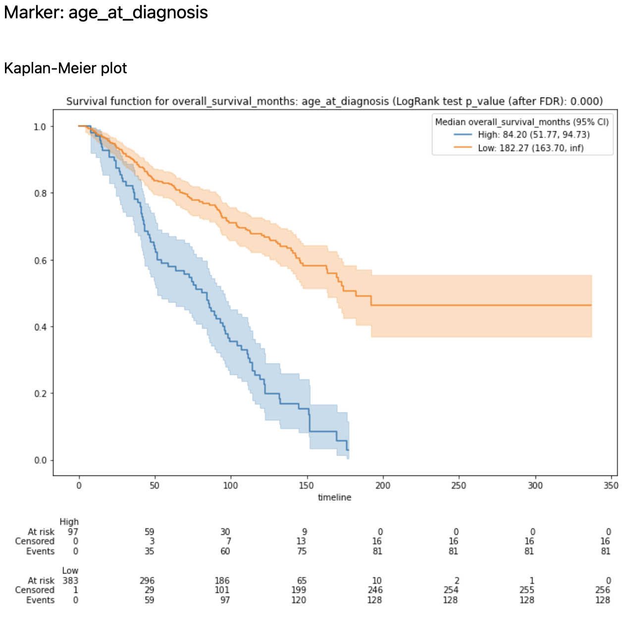
for a number of features (defined by n_plots_to_show parameter) Kaplan-Meier plots are created

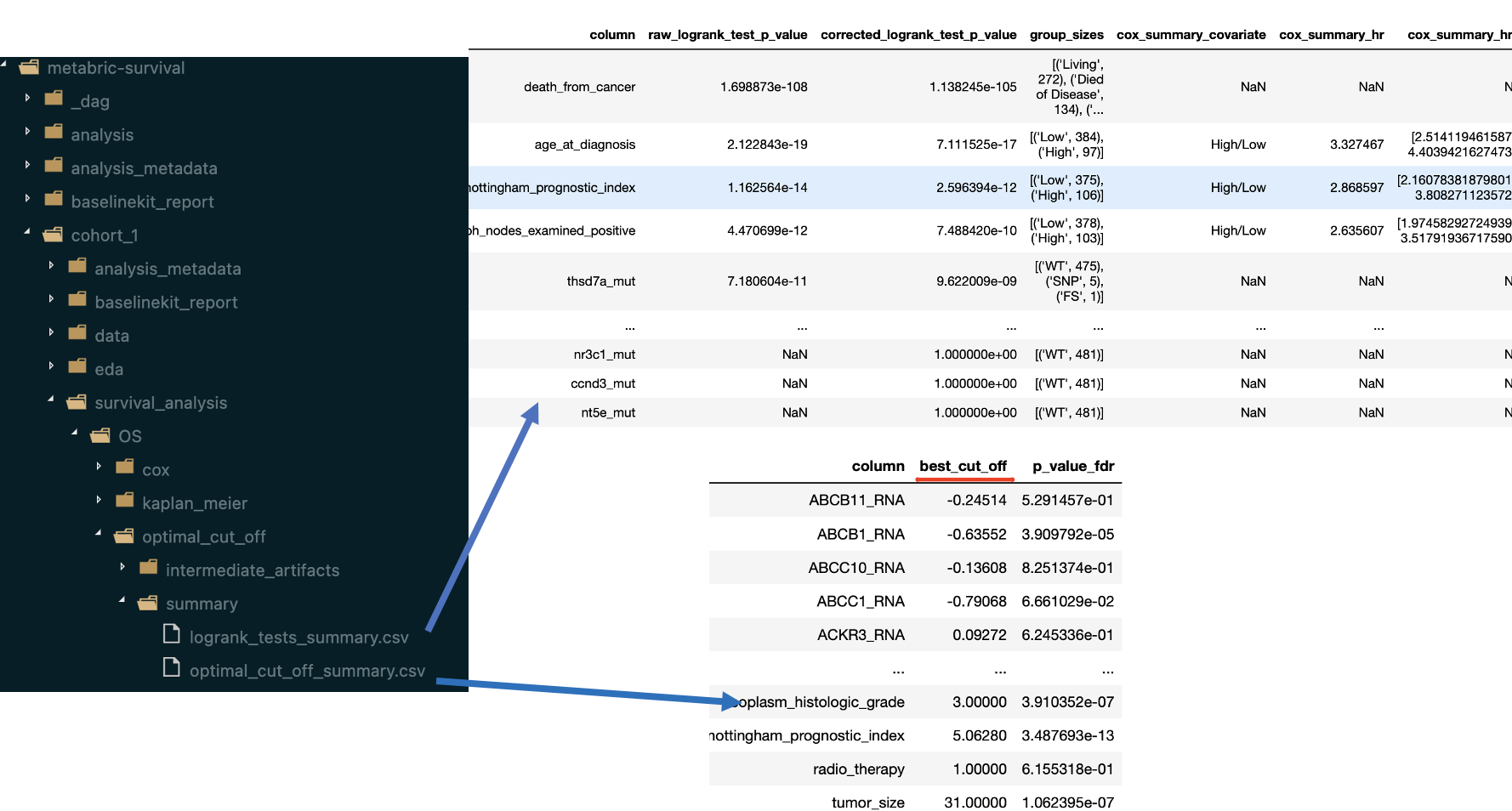
The summary table mentioned above can be found within dumped artifacts:

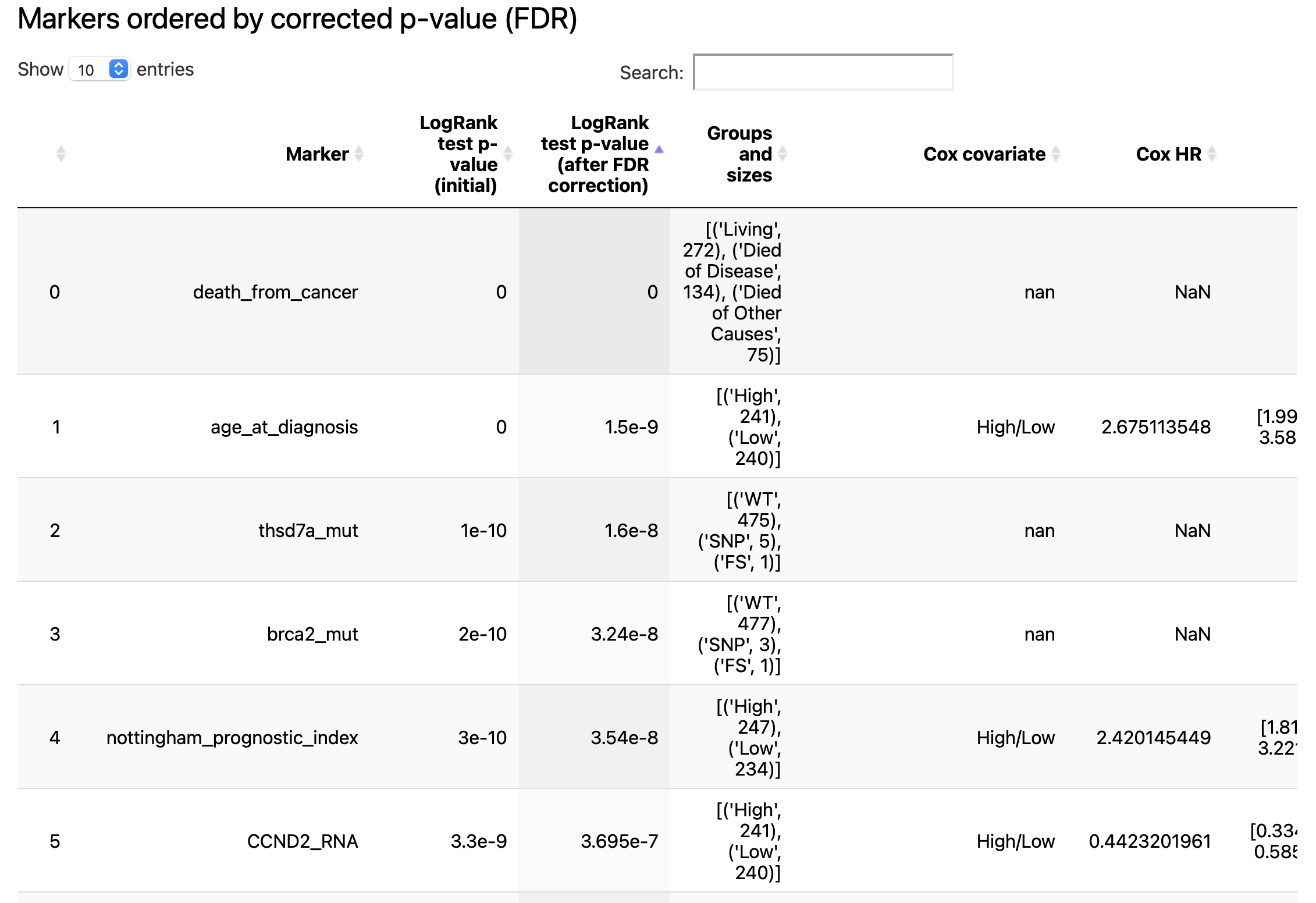
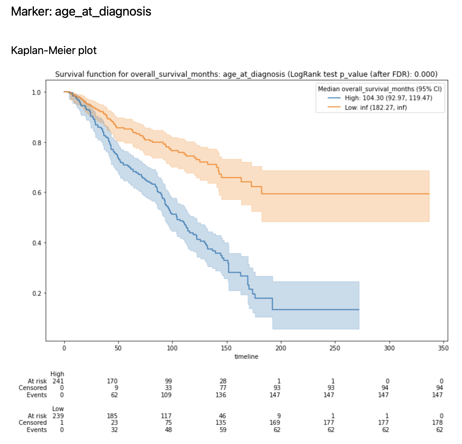
Optimal cut-off

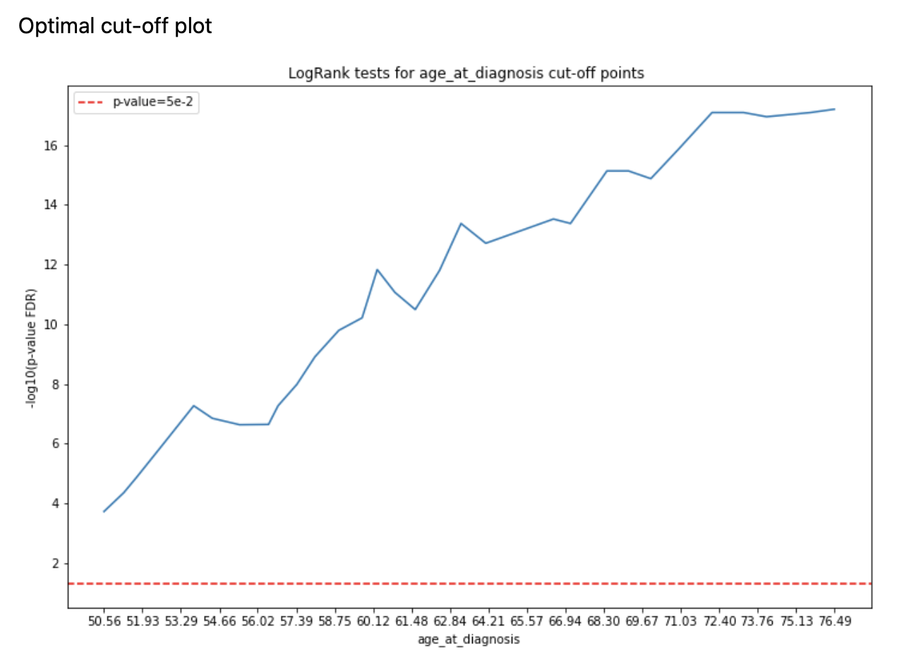
The method is based on the same schema as kaplan_meier method, the only difference is that for numerical features we want to find a better threshold rather than median under the following constraints (defined via logml.survival_analysis.extractors.optimal_cut_off.OptimalCutOffSAParams):

min_population - configures minimal fraction of samples within the smallest group (either ‘high’ or ‘low’), so that corner cases are avoided for which LogRank test returns unreasonable p-values
n_percentiles - number of potential threshold to check

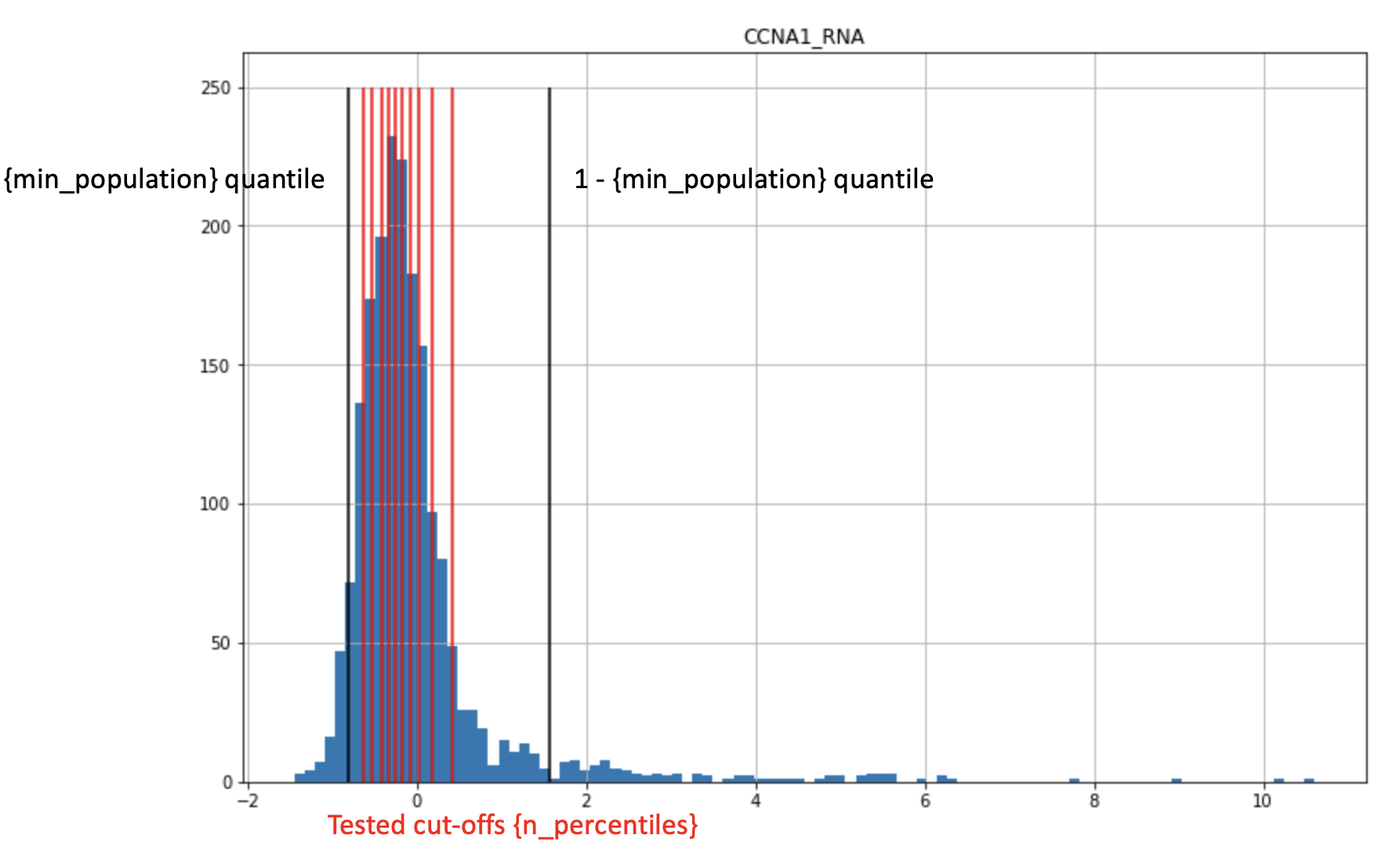
For all thresholds LogRank test is run and the best threshold is picked for a feature.

The result report contains the following artifacts:

table with features ranked by FDR-corrected p-values from LogRank tests

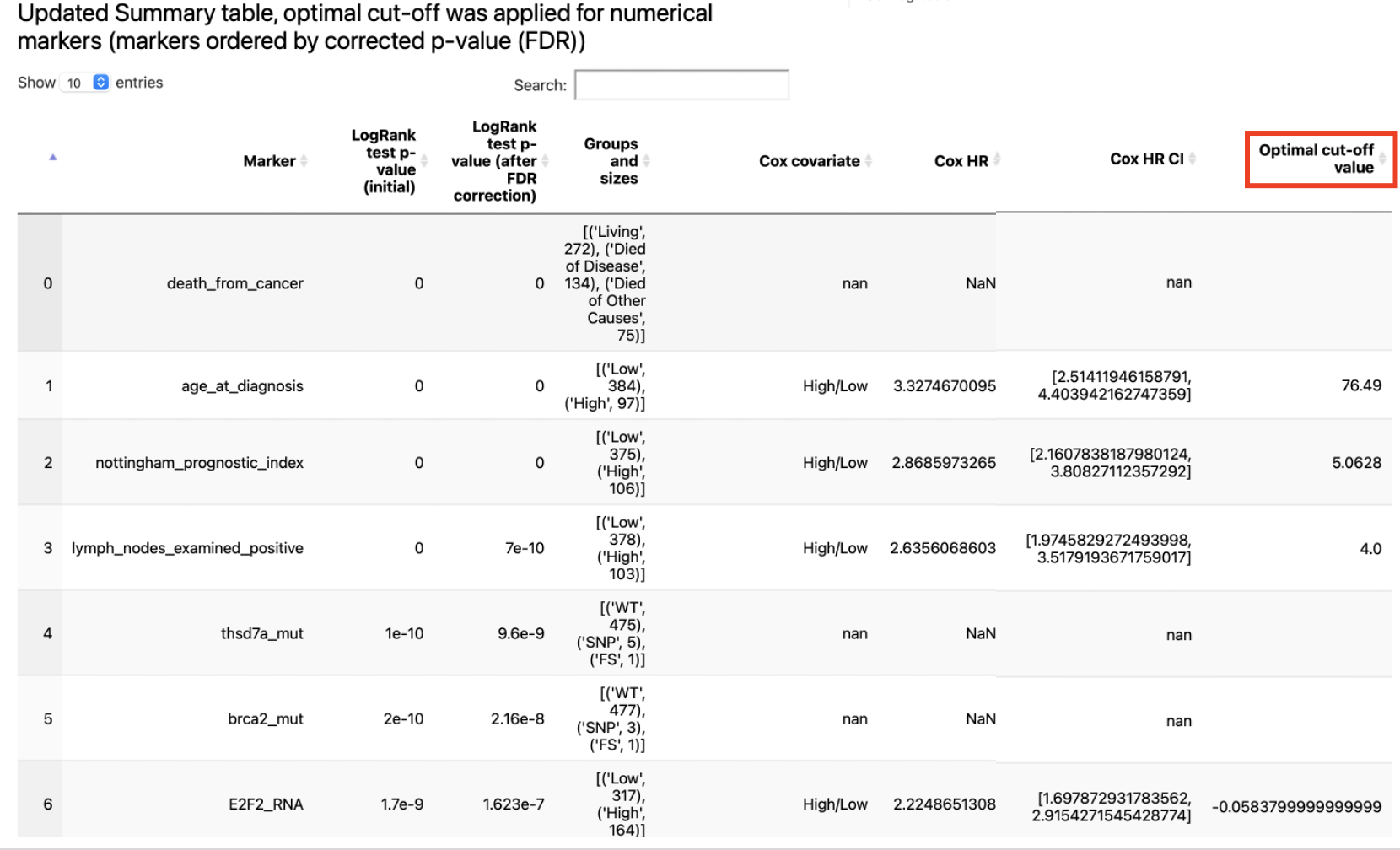
for a number of features (defined by n_plots_to_show parameter) Kaplan-Meier plots are created (using optimal cut-offs) and Optimal Cut-Off plot is created (with LogRank test results for candidate thresholds)

The summary table mentioned above can be found within dumped artifacts:

Multivariate methods

Data Preprocessing

Before applying multivariate analysis methods a given dataset is prepared by adding a few additional transformations to the preprocessing pipeline that was defined via configuration file:

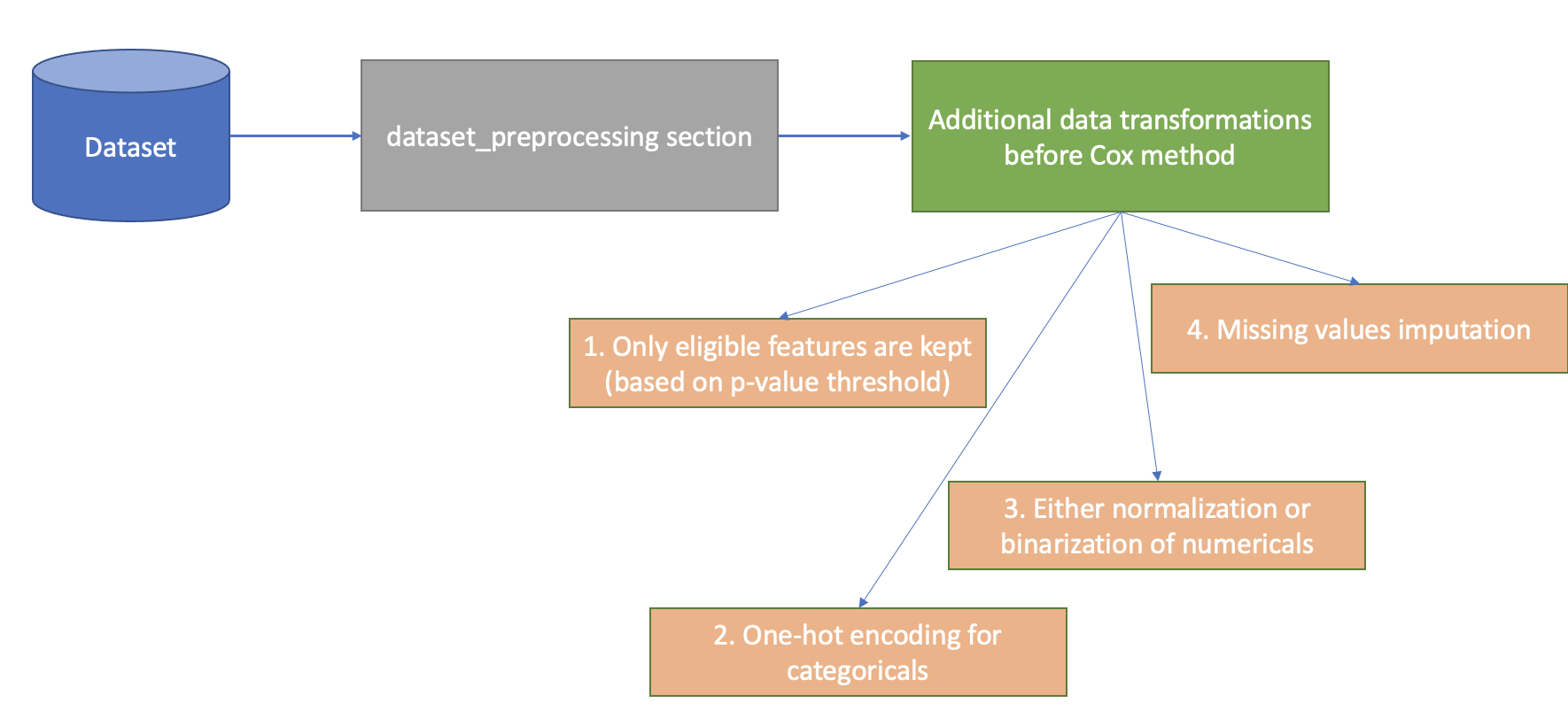
cox survival analysis method is strongly dependent on univariate methods, so the required prerequisite for running it is optimal_cut_off method. Based on univariate summary table the target set of features is defines via univariate_p_value_threshold parameter from logml.survival_analysis.extractors.cox.CoxSAParams - only features that are important enough in terms of univariate survival analysis (LogRank test p-value) are to be used in survival regression analysis (Cox).
normalize_numericals parameter defines whether numerical features should be normalized or based on the Optimal Cut-Off analysis results those features should be binarized (using best thresholds found).
all categorical features are one-hot encoded
all missing values are imputed using Iterative Imputation (MICE)

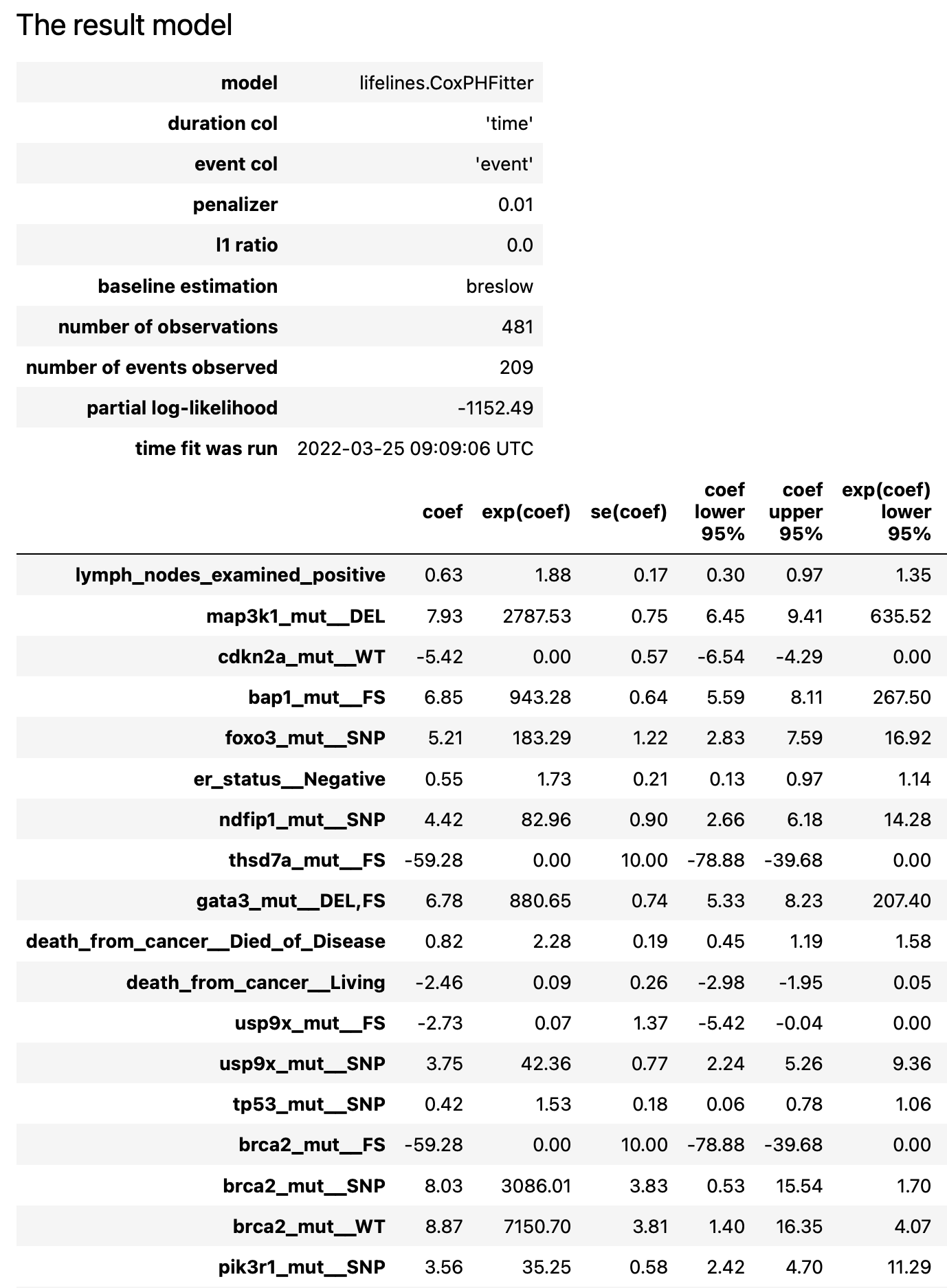
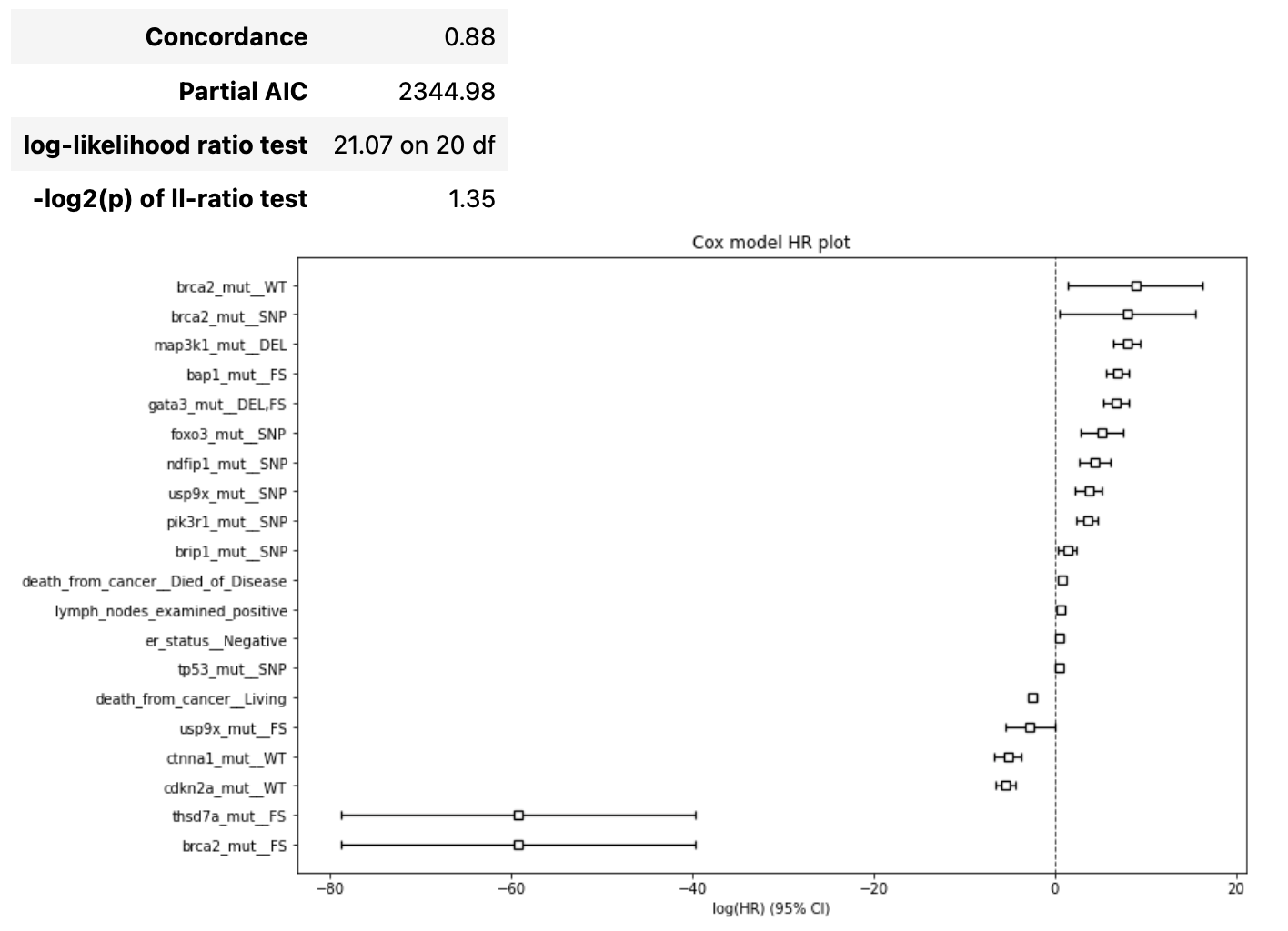
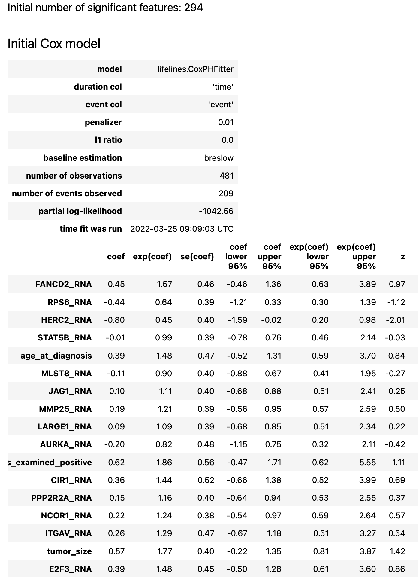
Cox backward-forward method

The method is based on the following paper - Cox backward-forward feature selection. The idea is to come up with a set of features for which a Cox regression model contains only significant features. There are two phases:

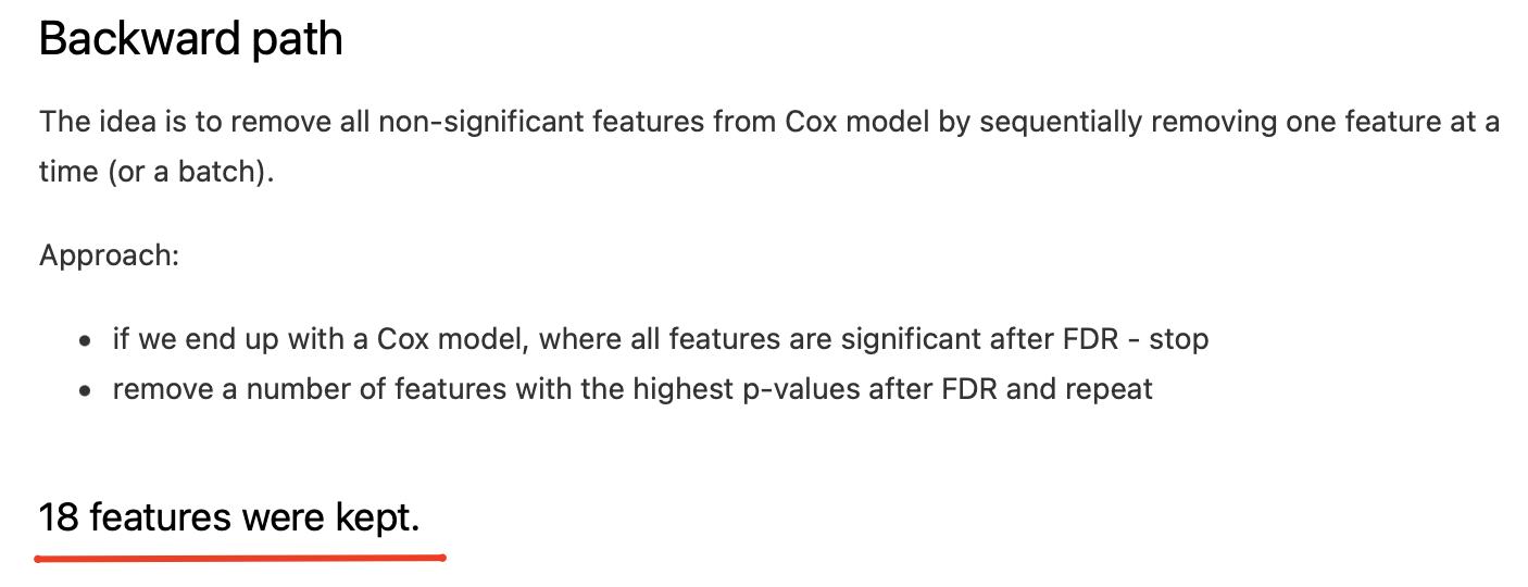
‘backward’ - until there are insignificant features based on current Cox model, those features are removed and a new Cox model is created
‘forward’ - features that were removed are sequentially (in reverse order) are added to Cox model, and if it makes sense - those are kept

The result report contains the following artifacts:

initial Cox model summary

details about forward/backward phases

result Cox model summary