Quick Start

Cond Environment

Install miniconda, then create the conda environment:

./scripts/env_create.sh
./scripts/env_update.sh

Check LogML :

conda activate logml

python log_ml.py --help

This generates the following output:

Usage: log_ml.py [OPTIONS] COMMAND [ARGS]...

Options:
  --help  Show this message and exit.

Commands:
  config            Configuration commands (Validation, schema, etc.)
  info              Print LogML version and environment info.
  models            Models commands.
  pipeline          Pipeline DAG commands.

So LogML is installed and available for launch.

First Run

Prepare for run

To run LogML you need:

• Dataset

• Logml configuration file

Dataset is a CSV file with a single line per sample/patient. It should contain covariates (free variables) and targets (dependent variables). Ultimate goal of LogML is to investigate connection between covariates and targets.

Covariates are usually a combination of clinical data and gene expressions, but also can be any other kind of data.

Targets usually are:

• Censored Survival time: Overall survival (OS), Progression-free survival (PFS).

• Treatment Response: Response rate or kind (complete, partial, etc).

Configuration file

Configuration file allows us to specifically parameters for analysis to be executed. It is a top level we specify set of sections which configure particular Analysis kind such as Modelling or Survival Analysis.

Next we prepare data and familiarise ourselves with the sample dataset.

Sample Dataset

LogML distribution includes a set of example datasets and configs which can be used for playing with LogML and understanding its basics. In this guide we’re using GBSG2 dataset.

Copy data and configs from LogML distribution to local folder:

cp -rvf ./examples ~/logml_examples
ls ~/logml_examples
head ~/logml_examples/gbsg2/GBSG2.csv

GBSG2 dataset

age	cens	estrec	horTh	menostat	pnodes	progrec	tgrade	time	tsize
70	1	66.0	no	Post	3.0	48.0	II	1814.0	21.0
56.0	1	77.0	yes	Post	7.0	61.0	II	2018.0	12.0
58.0	1	271.0	yes	Post	9.0	52.0	II	712.0	35.0
59.0	1	29.0	yes	Post	4.0	60.0	II	1807.0	17.0
73.0	1	65.0	no	Post	1.0	26.0	II	772.0	35.0

Sample Configuration File

Consider the simplest possible configuration file for exploratory data analysis of our sample dataset:

# ./log_ml.sh pipeline run -p gbsg2 -c examples/gbsg2/eda.yaml -d examples/gbsg2/GBSG2.csv -n gbsg2-eda

version:                     1.0.0

eda:
    params:
      correlation_threshold: 0.8

(We usually put example of logml command for launching it with this config file).

It is quite short and it asks LogML to produce EDA artifacts and then generate report.

Just in case, we validate config file:

log_ml.sh config validate ~/logml_examples/gbsg2/eda.yaml

OK: ~/logml_examples/gbsg2/eda.yaml is a valid config file.

At this point we know that the file is OK but in future it makes sense to validate it when you modify something manually.

Execute LogML

Now let’s run LogML to demonstrate this simple analysis.

log_ml.sh pipeline run --project-id gbsg2 \
    --config-path ~/logml_examples/gbsg2/eda.yaml \
    --dataset-path ~/logml_examples/gbsg2/GBSG2.csv \
    --output-path ~/logml_result  \
    --run-name gbsg2-eda

Let’s review this minimal set of parameters for logml to start working:

• –run-name which is gbsg2-eda in our case. Usually in real life this should follow some pre-defined schema, like (project-name)(stage)(date-time).

• –project-id: This is an indicator label, used to distinguish different projects.

• –config-path: Path to configuration file.

• –dataset-path: Path to dataset path. (Additionally we can provide path to a dataset metadata, but that’s out of scope of this guide).

• –output-path: Path to a root output folder. Specific output for the run will be available at {output path}/{run name}.

Warning

It is important to remember that output folder will contain parts of the original data, as well as intermediate files and reports. So output folder should be protected with the same access level as the data. In short, never put output data to public folders.

After we launch LogML, it will start processing, and generate quite amount of output. When it is finished, there is a final message about report readiness:

===============================================================================
Finished generating HTML for book.
Your book's HTML pages are here:
    ~/logml_result/gbsg2-eda/report/notebooks/_build/html/
You can look at your book by opening this file in a browser:
    ~/logml_result/gbsg2-eda/report/notebooks/_build/html/index.html
===============================================================================

Review Report

Now open the index.html file mentioned above: it is an entry point to the complete LogML report.

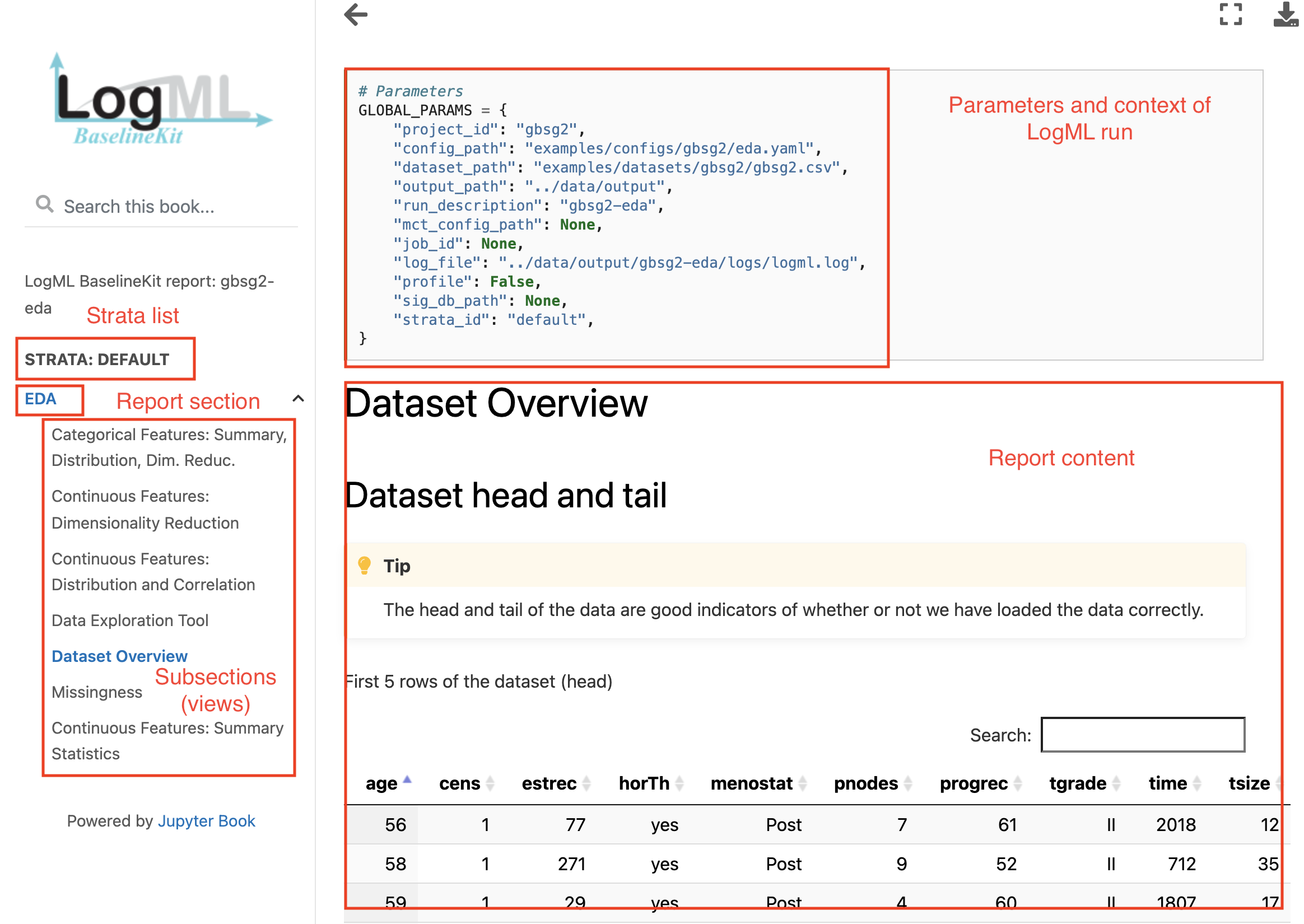
Report is organized in a top-down hierarchy with level:

• Stratum (Default in this case, which includes all the data).

• Analysis (EDA in our case. In case of modeling there is an instance per modeling problem)

• View (different aspects of the analysis. Most analyses have one view, EDA is quite diverse example).

First Survival Analysis

Let us now run some more interesting stuff: basic survival analysis. Consider the configuration file:

# ./log_ml.sh pipeline run -p gbsg2 -c examples/gbsg2/survival_analysis.yaml -d examples/gbsg2/GBSG2.csv -n gbsg2-survival-analysis

version:                    1.0.0

dataset_metadata:
    modeling_specs:
        OS:
            time_column:    time
            event_query:    'cens == 1'
            event_column:   cens

survival_analysis:
    problems:
        OS:
            methods:
                - method_id: kaplan_meier
                - method_id: optimal_cut_off
                - method_id: cox

You should notice several things here:

• We specify a dataset metadata, i.e. now we give columns special meaning. In the survival_specs section we created a Survival Specification named OS which declares time and event columns.

• Then we declare a problem for Survival Analysis. It is named OS too, which means that we also want to use survival specification named ‘OS’ here.

• Again, we ask ‘OS’ survival problem to be included into the report.

Now we run it:

log_ml.sh pipeline run --project-id gbsg2 \
    --config-path ~/logml_examples/gbsg2/survival_analysis.yaml \
    --dataset-path ~/logml_examples/gbsg2/GBSG2.csv \
    --output-path ~/logml_result  \
    --run-name gbsg2-sa

And again review the report, which contain Survival analysis report for “OS” problem.

This concludes a Quick start guide for LogML. We have walked through the environment, have found where to find and activate LogML distribution, examined basic LogML configuration files, and have ran two kinds of analysis for GBSG2 dataset.

Good luck, you’re now ready to explore LogML for your project.

Check other sections of this documentation for advanced topics.